“TX/RX schedules” tab
The TX/RX schedules tab contains the sheets with the coordinates of the generated TX and RX electrodes, with details on quadrupoles and measurements pseudo-plots.
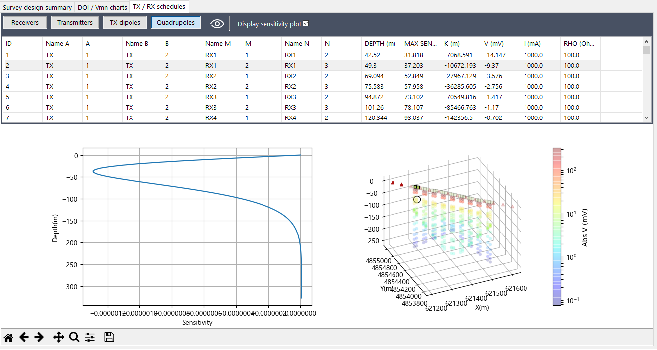
Fig. 29 Tab with sensor properties and pseudo-plots.
The tab consists of a topmost section with the toggle commands for selecting schedules to be displayed and a lower portion hosting the graphs.
Receivers schedule

Fig. 30 List with the properties of the receivers.
The list of the receivers contains information on the RX electrodes:
- V-FullWaver box identifier.
- Electrode number (1, 2 or 3).
- X, Y and Z UTM coordinates in meters.
- Geographic coordinates: longitude and latitude in degrees and decimals of degree.
Transmitters schedule

Fig. 31 List with the properties of the transmitters.
The list of transmitters contains information on the TX electrodes:
- Identifier of the group of transmitters (usually “TX”).
- Electrode number.
- X, Y and Z UTM coordinates in meters.
- Geographic coordinates: longitude and latitude in degrees and decimals of degree.
TX dipoles schedule

Fig. 32 List with the properties of the transmitting dipoles.
The list of TX dipoles contains information on the combinations of transmitters: the identification/number of the TX+ (A) electrode and of the TX- (B) electrode and a column with the dipole width in meters (length), useful for planning the TX cables arrangements.
Quadrupoles schedule
The list of quadrupoles contains information on the total set of TX/RX combinations:
- The four electrodes A, B, M and N that make up the quadrupole, indicated through the identifier/number pairs in the first eight columns of the table.
- The maximum depth of investigation of the quadrupole (in meters).
- The depth at which the maximum sensitivity of the quadrupole is recorded (in meters).
- The K geometric factor of the quadrupole.
- The expected Vmn signal (mV).
- The value of the injected current at TX (mA) which produces the potential Vmn at the receiving dipole.
- The apparent resistivity (Ohm m) for the measurement.

Fig. 33 List with the properties of quadrupoles.
The list of quadrupoles is the only one that has interactive features: selecting one table row allows to highlight the measurement in the pseudo-plot view: only the 4 electrodes of the quadrupole are colored and the measurement is emphasized by a highlighter circle. Remaining electrodes and measurements are represented in transparency. In addition, if the Display sensitivity plot checkbox is checked, the sensitivity plot for that quadrupole is shown. To remove the transparency of the quadrupoles from the graphs click on the command Refresh view of Fig. 34.
Fig. 34 Refresh view command.
Pseudo-plot

Fig. 35 Example of pseudo-plot.
The pseudo-plot sumarizes the salient features of quadrupoles in terms of coverage, depth of investigation and signal strength. The plot displays the position of the sensors (transmitters in red, receivers in green). The quadrupoles (colored points) are defined on the basis of the graphic properties described below.
- On the xy plane, the quadrupole is conventionally placed at the center of the RX dipole.
- The quadrupole is placed at the z depth corresponding to the maximum depth of investigation.
- The color scale assigned to the measurements is the one defined by the range of absolute values of the Vmn signal.
Sensitivity plot for the quadrupole

Fig. 36 Example of sensitivity plot.
This plot shows the behavior of the sensitivity of quadrupole with depth. This is the function that is integrated for the calculation of the maximum depth of investigation.