“DOI/Vmn charts” tab
The DOI/Vmn charts tab allows to explore the values for maximum sensitivity and depth of investigation for the different combinations of receiving and transmitting dipoles and to check how the Vmn signal changes when the background resistivity or the input current is modified.
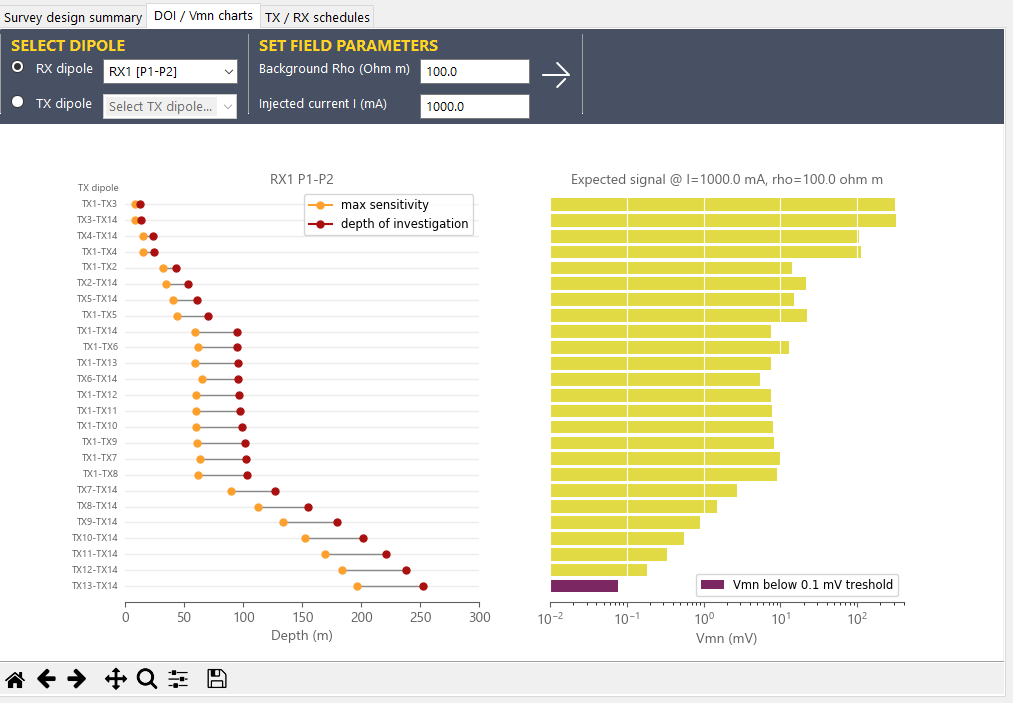
Fig. 28 Charts with maximum sensitivity, depth of investigation and expected Vmn signal.
The tab consists of a horizontal bar at the top, where the commands for analysis are hosted, and two graphs, one for maximum sensitivity/depth of investigation (left in Fig. 28) and one for potential Vmn (right).
Select dipole
This section allows to select the dipole used to perform the analysis. You can choose between two modes:
- RX dipole: allows to perform the analysis on a specific receiving dipole. Calculates the maximum sensitivity, depth of investigation and potential Vmn related to all transmitting dipoles in combination with that specific RX dipole. Example in Fig. 28 represents this mode for the dipole made up of the P1 and P2 electrodes of the V-FullWaver box named RX1.
- TX dipole: allows to perform the analysis on a specific transmitting dipole. Calculates the maximum sensitivity, depth of investigation and potential Vmn related to all receiving dipoles in combination with that specific TX dipole.
Set field parameters
The parameters here are related to the fieldwork scenario:
- Background Rho: this is the value (in Ohm m) of the site background resistivity.
- Injected current: this is the value (in mA) the user supposes will be able to inject into the ground at the transmitting dipoles.
To make the changes effective, click on the arrow button Apply. The defaults (100 Ohms m and 1000 mA) can be changed in the Field parameters section of the Preferences panel.
Sensitivity/depth of investigation chart
This plot represents the values of maximum sensitivity (orange marker) and of maximum depth of investigation (red marker) for each combination of TX/RX dipoles. Positioning the mouse pointer inside the graph allows to view (horizontal bar at the top-right) the value of the z depth in meters at the selected point.
The depth of investigation estimate is performed, first, integrating the analytic sensitivity function – for the given quadrupole – and then by calculating the median z depth, so that the area under the sensitivity curve is equal to the 50% of the total area (Edwards, 1977 [1] ; Baker, 1991 [2] ).
Note
For peculiar arrangements of the transmitting and receiving electrodes, in particular when the two dipoles are strongly orthogonal, the sensitivity curve with depth can change of sign and show multiple local extremes, which can make sometimes not very reliable the estimate of the depth of investigation. For these particular quadrupoles, or for models that take into account complex scenarios of 3D distribution of resistivity, or, again, in case of marked topographic variations, it may be useful to save the project to DATA file through the command Save project of the Open and save project panel and perform a specific modeling with advanced tools, such as the ERTLab64 TM software.
Vmn signal graph
This plot represents the expected Vmn potential (in milliVolt) for each combination of the TX/RX dipoles. The scale of representation of potentials is logarithmic. The bars are green if the (absolute) value of Vmn is between the minimum and maximum thresholds specified in the Field parameters section of the Preferences panel. For signals below the minimum threshold the bar turns purple, as displayed in Fig. 28 : in the example this happens for the P1-P2 dipole of RX1 box for the TX13-TX14 transmission dipole. Similarly, for signals above the maximum threshold (overload risk at the receiver) the bar turns to red. Positioning the mouse pointer inside the graph allows to view (horizontal bar at top-right) the value of the potential Vmn in milliVolt at the selected point.
Footnotes
| [1] | L.S. Edwards, 1977. A modified pseudosection for resistivity and induced-polarization. Geophysics, 42, 1020-1036. |
| [2] | Barker, R.D., 1991. Depth of investigation of collinear symmetrical four-electrode arrays. Geophysics, 54, 1031-1037. |